- Webanwendung, zum Erstellen und für die gemeinsame Nutzung von Dokumenten, die sowohl Live-Code, Gleichungen, Visualisierungen, Links als auch formatierten Text enthalten
- ideales Werkzeuge, um Programme, ihre Ergebnisse und ihre Beschreibung und Dokumentation zu vereinen und die Datenanalyse in Echtzeit durchzuführen
"Jupyter" - Acronym für die umgesetzten Haupt-Programmiersprachen Julia, python und R; unterstützt heute viele andere Sprachen
Im Browser-Fenster:
- Startseite der Anwendung mit Liste der Notebooks

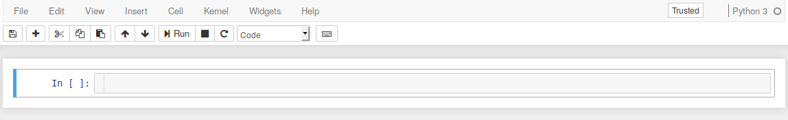
- Folge (mehrzeiliger) Text-Eingabe-Felder für
- Überschriften
- Code
- Kommentare
- Programm-Ausgaben
sowie Steuerelementen für die Ausführung von Code
Start der Anwendung erfolgt im Terminal-Fenster (im Ordner mit Notebooks):
jupyter notebook
bzw. Start eines bestimmten Notebooks:
jupyter notebook notebookname.ipynb
öffnet Browser-Fenster mit der Adresse: http://localhost:8888
Beim Anlegen eines neuen Dokuments:
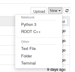 Auswahl von Python 3 (= jupyter notebook), Text File, Folder oder Terminal
%matplotlib inline
%pylab inline
Neben Code-Zellen gibt es die Möglichkeit, Zellen vom Typ Markdown für die Dokumentation zu verwenden.
Markdown ist eine Auszeichnungssprache (wie html) für einfache Textgestaltung mit
- ###### Überschriften
- Textformatierung
- kursiv
- fett
- kursiv und fett
- Listen
- Geordnet
- Ungeordnet
- Blockzitate
- Interne und externe Links
- Blockzitate
- Code-Abschnitte
str="Das ist eine Codezeile."
print(str)
- Tabellen
- Bilder
- mathematische Symbole $(\LaTeX)$ und ∃ UTF-8 Mathematische Operatoren
- Zeilenumbrüche und horizontale Linien
Magic functions
%lsmagic
%ls
%quickref
Betriebssystem-Befehle:
!pwd
python-help:
?range
Zeitmessung (eine Code-Zeile):
%time x = range(100)
Zeitmessung (mehrzeilig):
%%timeit x = range(100)
    mean(x)
?%%timeit
%%HTML
<img src="https://www.python.org/static/img/python-logo.png">
<p>Jupyter kann HTML rendern!</p>
Jupyter kann HTML rendern!
$\LaTeX$ im Fließtext und in abgesetzten Formelzeilen $$\LaTeX$$ in Markdown sowie in Code Zellen:
%%latex
\begin{align}
\vec{M} = \vec{r}\times\vec{F} =
\begin{vmatrix}
\vec{e}_x & \vec{e}_y & \vec{e}_z \\
x & y & z \\
F_x & F_y & F_z
\end{vmatrix}
\end{align}
Nutzer-interaktion mit widgets
from ipywidgets import interact, fixed

def f(x):
    print(x)

interact(f, x=(2, 20, 2));
interact(f, x=False);
interact(f, x="Text!");
def plotsin(omega):
    t = arange(0, 1, 0.01)
    plt.plot(t, sin(omega*t))
    plt.show()

interact(plotsin, omega=(0.1, 10*pi, 0.1));
Das Display System
Universelles Werkzeug zur Anzeige verschiedener Darstellungen von Objekten.
Der Aufruf von display für ein Objekt sendet alle möglichen Darstellungen des Objekts an das Notebook. Diese Darstellungen werden im Notebook-Dokument gespeichert. Im Allgemeinen verwendet das Notebook die reichhaltigste verfügbare Darstellung. Für konkrete Darstellungen (html, latex, jpeg, png, svg, json) gibt es entsprechende Funktionen.
Bilddarstellung aus
- Rohdaten oder URL:
from IPython.display import display, Image
Image(url='http://python.org/images/python-logo.gif')
- lokalen Dateien:
img = Image(filename="images/python.png")
display(img)

- Vektorgrafik (SVG):
from IPython.display import SVG
SVG(filename='images/jupyter-logo.svg')
Audio:
import numpy as np
from IPython.display import Audio
f1, f2 = 500, 505
dauer, rate = 5, 6000
t = np.linspace(0, dauer, dauer*rate)
signal = np.sin(2*np.pi*f1*t) + np.sin(2*np.pi*f2*t)

Audio(data=signal, rate=rate)
Video:
from IPython.display import Video
Video("images/Kreisbahn.mp4")
from IPython.display import YouTubeVideo
YouTubeVideo("ZN2vAQmy4nk")
Links zu lokalen Dateien:
from IPython.display import FileLink, FileLinks
FileLink('jupyter-notebook.ipynb')
FileLinks(".")
Einbinden externer Webseiten:
from IPython.display import IFrame
IFrame('https://jupyter.org/', width='100%', height=400)
$\mathbf{\LaTeX}$:
from IPython.display import Math
Math(r'F(k) = \int_{-\infty}^{\infty} f(x) e^{2\pi i k} dx')
from IPython.display import Latex
Latex(r"""
\begin{align}
\epsilon_0 \nabla \cdot \vec{\mathbf{E}} & = \varrho \\
\nabla \times \vec{\mathbf{E}}\, + \, \dot{\vec{\mathbf{B}}} & = \vec{\mathbf{0}} \\
\nabla \cdot \vec{\mathbf{B}} & = 0 \\
\frac{1}{\mu_0}\nabla \times \vec{\mathbf{B}} -\, \epsilon_0 \dot{\vec{\mathbf{E}}} & = \vec{\mathbf{j}}
\end{align}
""")
Notebook Inhalte exportieren
jupyter nbconvert --to html jupyter-notebook.ipynb
jupyter nbconvert --to pdf jupyter-notebook.ipynb